I make it no secret to those who know me that I am an avid lover of music; so, it is only natural that I incorporate my interests into other parts of my life.

As a beginner in the perplexing world of Big Data and someone who only started learning to code with Python for four months, I decided to stick to things I enjoy and do something related to music for my first school-related project. After much searching, I found a dataset — found at https://www.kaggle.com/insiyeah/musicfeatures — that used the LibROSA package (a Python package for analyzing music and other audio alike) to grab features from about 1200 songs with ten different genres: blues, classical, country, disco, hip hop, jazz, metal, pop, reggae, and rock. While every feature I used contained continuous floats and integers, my target feature had a finite amount of options therefore, it was best to use a classifier to go about my predictions.

Before proceeding to models, I first had to clean up my data. The first big issue I came across was the mislabeling of 200 observations in the label column as integers and not a string containing a genre.

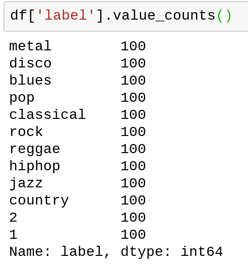
To fix this, I was able to find the genres listed in the column ‘filename’ so I went ahead and made a column called ‘genre’ to fix this issue and then enumerated them using the OrdinalEncoder from Category Encoders. Unfortunately, in doing this, I ended up with an unequal distribution of genre observations (100 additional classical and pop songs).

for _ in df[‘filename’]:
 genres.append(_[:-9])</span><span id="2e9a" class="fb hw hx ef hy b de ic id ie if ig ia w ib">df.insert(1, ‘genre’, genres)</span>

Now that I was happy with the dataset, I split the data up into the train, validate and test data frames using sci-kit learn and made a function to wrangle the data into their corresponding X and Y matrices — now, onto finding a model.

I decided to play around with different models we used in class including DecisionTreeClassifier and RandomForestClassifier and adjusted the parameters. I found DecisionTreeClassifier to yield some pretty poor results at about 59% accuracy however, RandomForestClassifier was able to produce an accuracy of 70% with default parameters when coupled with StandardScaler from sci-kit learn.

Hoping I could further push the score of my model, I decided to play around with the parameters of Standard Scaler and Random Forest Classifier using RandomizedSearch Cross-Validation. I was showing off a bit, in the beginning, performing ten cross-validations with 100 iterations — as this was my first time using a local setup — but that was probably very unnecessary; in any case, I still was only able to obtain a 69% accuracy even after all of those fits. To save time for those who wanted to run my code (seen below), I reduced the total fits to about 40 over the same parameter distribution.

from sklearn.model_selection import GridSearchCV, RandomizedSearchCV
from scipy.stats import randint, uniform</span><span id="391f" class="fb hw hx ef hy b de ic id ie if ig ia w ib">param_distributions = {
 ‘standardscaler__with_mean’: [True, False],
 ‘standardscaler__with_std’: [True, False],
 ‘randomforestclassifier__n_estimators’: randint(50,500),
 ‘randomforestclassifier__max_depth’: [5,10,15,20,None],
 ‘randomforestclassifier__max_features’: [None, ‘auto’, ‘log2’],
}</span><span id="b2e3" class="fb hw hx ef hy b de ic id ie if ig ia w ib">search = RandomizedSearchCV(
 pipeline,
 param_distributions=param_distributions,
 n_iter=10,
 cv=4,
 scoring=’accuracy’,
 verbose=10,
 return_train_score=True,
 n_jobs=-1
)</span><span id="ae62" class="fb hw hx ef hy b de ic id ie if ig ia w ib">search.fit(X_train, y_train);</span>

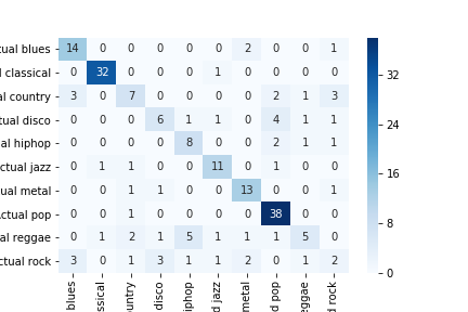
To visualize my model’s accuracy, I created a confusion matrix using the model with the highest accuracy. In class, we were able to ‘pretty up’, as it were, the bland matrix that is returned when using the confusion_matrix function from sklearn.metrics and since I had great difficulty producing visuals for prior models, I felt it was necessary to have something. The code below shows the function used to visualize the matrix using the heatmap option in Seaborn followed by the output (unfortunately some words were cut in attempting to save the image using fig.savefit() — the Y-axis represents the actual genre and the X-axis represents the predicted genre)

from sklearn.utils.multiclass import unique_labels
from sklearn.metrics import confusion_matrix</span><span id="7d8d" class="fb hw hx ef hy b de ic id ie if ig ia w ib">def plot_confusion_matrix(y_true, y_pred):
 labels = unique_labels(y_true)
 columns = [f’Predicted {label}’ for label in labels]
 index = [f’Actual {label}’ for label in labels]
 df = pd.DataFrame(confusion_matrix(y_true, y_pred),
 columns=columns, index=index)
 return sns.heatmap(df, annot=True, fmt=’d’, cmap=’Blues’)</span><span id="cb02" class="fb hw hx ef hy b de ic id ie if ig ia w ib">pipeline = make_pipeline(
 StandardScaler(),
 RandomForestClassifier(n_estimators=100, random_state=42)
)
pipeline.fit(X_train, np.ravel(y_train))</span><span id="36fa" class="fb hw hx ef hy b de ic id ie if ig ia w ib">y_pred = pipeline.predict(X_val)
plot = plot_confusion_matrix(y_val, y_pred)</span>

While I was satisfied with the score of my model, I wanted to get the most out of what I learned; so, I wanted to check feature importance using Permutation Importance and subsequently visualize it using eli5.

As learned in class, I assigned a variable ‘permuter’ to Permutation Importance and passed through my model to predict accuracy score over five iterations. When I used the show_weights() function, I was able to find 2 features that had little importance to my model so, using a mask, I was able to remove the features that had a permutation importance of less than zero and further increase my accuracy score to 72% — I have included the weights of each feature from my dataset below.

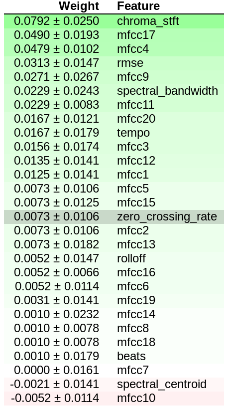
My model achieved higher accuracy without the features ‘spectral_centroid’ and ‘mfcc10’

In the end, I was pretty happy with what I achieved. I was surprised my model’s accuracy was higher than a coin toss. The main doubt I had in tackling this project was that I was leaving it up to a machine-learning algorithm to know something about music appreciation, that is, understanding what they are hearing and be able to tell what genre a song is labeled. For me, I probably have a different idea of what genre a song is compared to that of my colleagues; for instance, the genre ‘classical’ for someone could mean any song (or piece) played by an orchestra when it is music from a specific era (mid 17th C to early 18th C). Regardless, this project topic was a very interesting choice and I am looking forward to future projects using data from other disciplines.